一个古早的天气预测方法

这是随机信号分析四篇课程报告之一，也是我认为较有意思的一篇报告。主要内容是复现一篇与课程内容有关的论文。这篇论文使用卡尔曼滤波预测未来几天天气。

天气递推系统

系统假设

动态噪声与测量噪声都是随机向量，假定它们是互不相关的、均值为零、方差分别为 $W$, $V$ 的白噪声
一段时间内未发生突然性的天气变化因素，即引起天气变化的因素渐进变化。

卡尔曼滤波递推系统

卡尔曼滤波用于天气预报时，根据陆如华等人研究[1]，考虑到假设中由季节等原因所引起的
$B$ 变化是渐进的，且有随机性，采用状态方程的简化形式：
$$B_t = B_{t−1} + \epsilon_{t−1}$$ 其中： $B_t$ 及 $B_{t−1}$ 是 $t$ 及 $t-1$ 时刻的值$\epsilon_{t−1}$ 是动态噪声。

至于测量方程，可将回归方程作为 KF 中的测量方程。测量方程的形式：
$$Y_t = X_tB_t + e_t $$ 其中： $Y_t$ 是预报量( °C) ,$X_t$ 是因子矩阵,$B_t$ 是回归系数 $e_t$ 是测量噪声。

动态噪声与测量噪声都是随机向量，假定它们是互不相关的、均值为零、方差分别为$W$, $V$ 的白噪声，得到 KF 的递推系统：

$\hat{Y_t}$ 是$t$时刻的温度预测量，$X_t$ 是$t$时刻的观测因子测量值，$\hat{B_{t-1}}$是上一时刻的观测因子的回归系数矩阵。 $$\hat{Y_t} = X_t \hat{B_{t-1}}
$$
由于回归系数矩阵具有误差，因此状态方程的总误差为回归系数矩阵方差$C_{t-1}$与动态噪声方差$W$之和：
$$R_t = C_{t−1} + W$$
测量方程的误差方阵为状态方程方差阵经过测量因子$X_k$的变换后加上测量误差方阵$V$
$$\sigma_t = X_tR_t X_t^T + V$$ 得到卡尔曼增益: $$H_t = R_t X_t^T\sigma_t^{-1}
$$
根据温度的实测值和上一时刻的回归系数矩阵，得到下一时刻的回归系数矩阵
$$\hat{B_t} = \hat{B_{t-1}} + K_t(Y_t −\hat{Y_t})$$
最后更新回归系数矩阵的误差方差阵： $$C_t = R_t − H_t\sigma_t K_t^T$$

参数说明

收集到的天气数据共有两类，一类是地球表面数据，另一类是高空气象数据。
表面数据：

    数据类型           符号                  说明

      温度             $T$                摄氏度 °C
      相对             $H$               空气相对湿度
   海平面压力         $SLP$               帕斯卡 Pa
      风速           $W_{sp}$        千米每小时 km h^−1^
  云覆盖数据：      $CL,CM,CH$   天空覆盖低、中、高云的百分比

压力所在的位势高度 $h$ 米 m
位势高度500m处温度 $T_{500}$ 摄氏度 °C
位势高度850m处温度 $T_{850}$ 摄氏度 °C
位势高度500m处压强 $P_{500}$ 帕斯卡 Pa
位势高度850m处压强 $P_{850}$ 帕斯卡 Pa

根据地表温度，空气相对湿度，海平面压力和地面风速作为因子，选择蒙古乌里雅苏台4月13日00UTC至4月29日21UTC每三小时为单位的天气数据进行数据拟合。

如图 [1] 所示为蒙古乌里雅苏台4月13日至4月29日的气温，风速，空气相对湿度以及气压数据。根据数据拟合得到曲线。

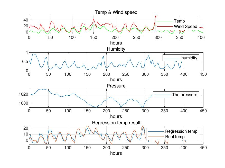
图1：蒙古乌利雅苏台短期天气情况及其回归曲线

观测方程以及初值的确定

卡尔曼滤波运行前对于初值 $B_0$、$C_0$以及 $W$ 和 $V$
都要事先确定，由拟合曲线可知， $$B_0 =
\begin{bmatrix}
-20.990\
0.303\
0.009\
\end{bmatrix}$$

$C_0$ 是 $B_0$ 的误差方差阵，由于 $B_0$ 是从样本资料精确计算得到的，可以假定它与理论值相等，即认为回归系数的初值为系统真值，则其误差方差为零。所以$C_0$ 是 $3 \times 3$的零方阵。

由于 $W$ 和 $V$ 在进行 KF 运算起始时被确定之后就不能再改变，因此需先计算出 $W$ 和 $V$ 的值。根据陆如华等人研究，$n$ 个因子的系统中 $W$ 由式决定 $$W \approxeq
\begin{bmatrix}
\frac{(\Delta B_1)^2}{T} & 0 & \dots & 0 \
0 & \frac{(\Delta B_2)^2}{T} & \dots & 0 \
\vdots & \vdots & \vdots & \vdots \
0 & 0 & \dots & \frac{(\Delta B_n)^2}{T} \
\end{bmatrix}
$$ 由上式可见，$W$ 值可用 $B$ 的变化来估算，因此需进行另一次拟合计算，时段取4月13日00UTC至5月9日12UTC，求出$B_t$ ， $$B_t =
\begin{bmatrix}
-26.161 \
0.283 \
0.012 \
\end{bmatrix}$$ 由 $B_0$ 和 $B_t$ 的时间间隔 $\Delta T = 28$，因此可求出 $W$ 的近似值为 $$W =
\begin{bmatrix}
0.35 & 0 & 0 \
0 & 5.10e-06 & 0 \
0 & 0 & 1.51e-07 \
\end{bmatrix}$$ 长期天气情况及其拟合曲线如图[2]所示。

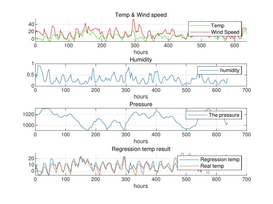
图2：长期天气情况及其回归曲线

至于测量噪声的方差，根据陆如华等人研究
$$V = \frac{q}{k -m -1}$$

其中 $q = \sum_{k=1}^{k} (y_i-\hat{y_i})^2$;$k$ 为样本容量;$m$为量测方程因子数;$y_i$ 为观测值;$\hat{y_i}$为回归方程估算值

最后求出$V = 16.63$

预测结果

卡尔曼滤波初始参数确定后，在 5 月 10 日 00UTC
开始作不断更新及预报,分别得到短期卡尔曼天气预测结果和长期卡尔曼天气预测结果。

短期预测结果

从短期结果来看，卡尔曼滤波系统得到的天气预测值与实际观测值在总体趋势上保持一致。在0 5h和18 28h的气温下降段，预测值也呈现出明显的下降趋势。

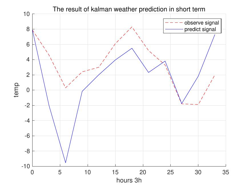
图3：短期天气预测

长期预测结果

从长期结果来看，卡尔曼滤波系统得到的天气预测值与实际观测值在总体趋势上保持一致。在多个实际的气温下降段，预测值也呈现出明显的下降趋势。

但是从图 [4] 中不难看出，预测值存在过冲现象，即在气温的多个极值点处，预测温度均高于或低于实际测量温度。

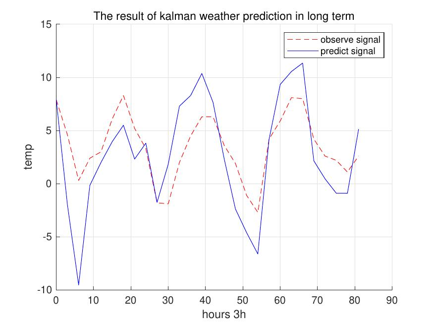
图4：长期天气预测

讨论

测量协方差的调校

通过改变量测噪声方差 $V$ 的值可以对 KF 的特性作出调整，由式可知，如果将量测噪声方差$V$增大，那么 KF 将不太相信实测值，而 $H_t$ 相应会减小，进而影响到回归系数的值，最后使滤波结果较慢去反应实测气温的变化；测量噪声方差减少时，KF 将较相信实测值，滤波结果将较快去反应实测气温的变化。因此对 $V$ 的值进行调校，进行两个设定的试验，第一个为快反应设定，取 $V/1000$，这是较快反应实测值的变化；第二个为慢反应设定，取 $V*1000$，这是较慢反应实测值的变化

实际过程中不断地调整$V$的数值从$1e-4V$到$1e+4V$ ,一共绘制出九条曲线。分别对长期天气预测结果和短期天气预测结果进行分析。图[5]与图[6]中最佳预测曲线使用红色进行标注。

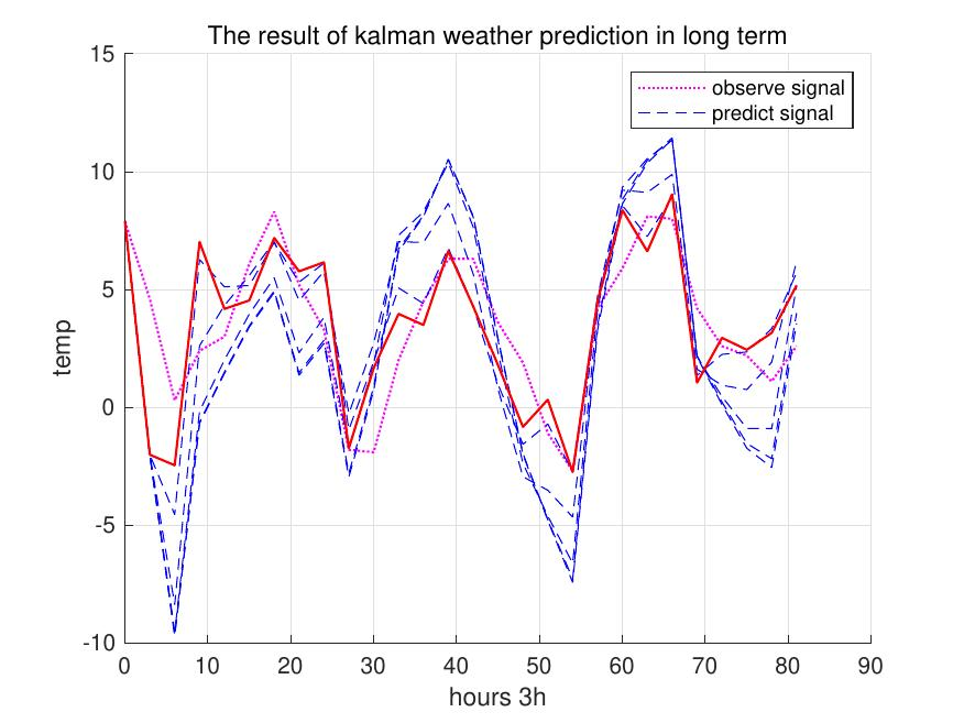
图5：长期快慢反应卡尔曼预测

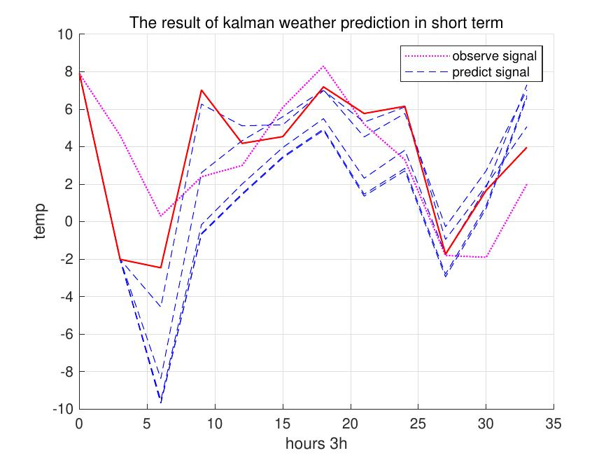
图6：短期快慢反应卡尔曼预测

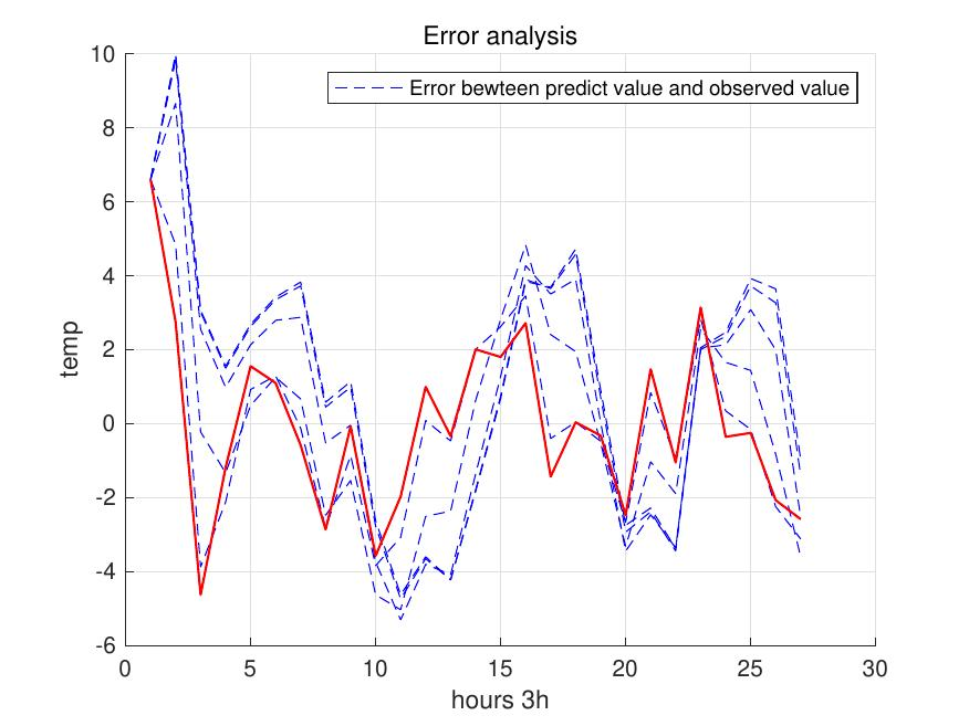
图7：误差比较

从最后的误差来看，快反应 KF 对天气实际情况的预测效果最好。

参数选取

由于实际过程中影响天气的因素很多，仅仅使用三个因子对天气情况进行预测不稳定性较大。增加天气因子至十个：地表温度，空气相对湿度，地表气压，低空云层覆盖率，中空云层覆盖率，高空云层覆盖率，500米位势温度，500米位势气压，850米位势温度以及850米位势气压。

再次进行拟合分析得到结果如图[8]和图[9]示。

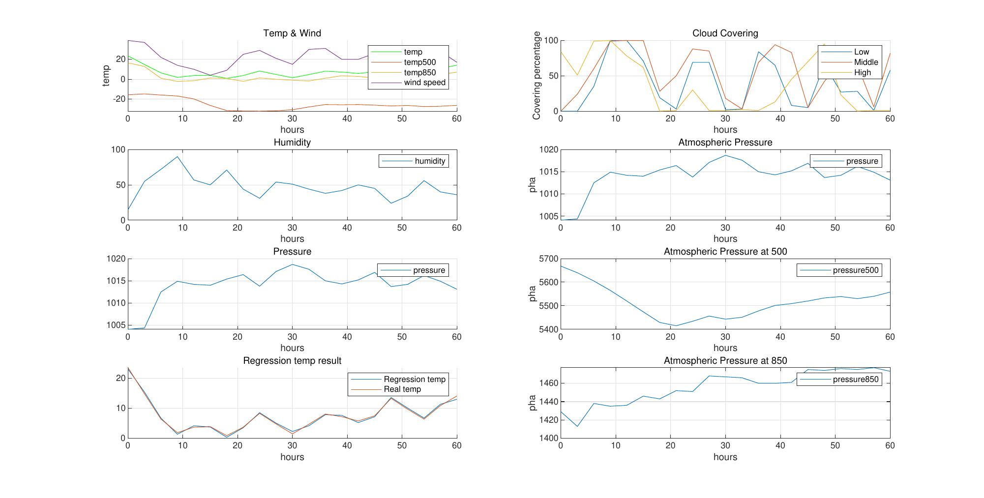
图8：增加因子选取范围后短期回归

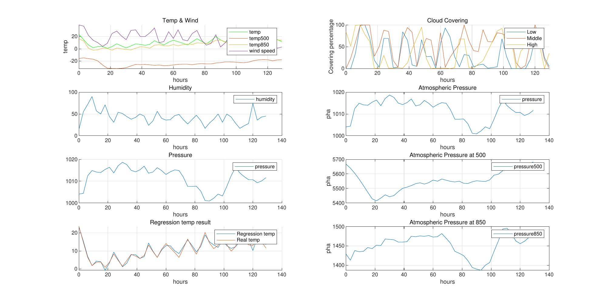
图9：增加因子选取范围后长期回归

再次建立 KF 递推系统进行分析，得到长期天气预测数据如图[10]

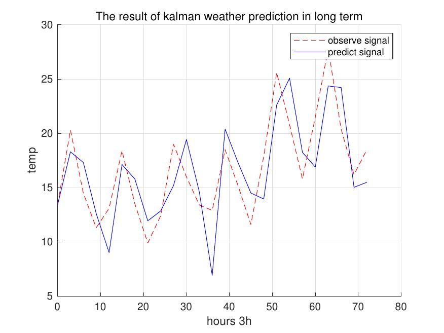
图10：长期天气情况预测

该方法预测结果的绝对值平均误差为2.80°C 与三因子方法绝对值平均误差在快反应 KF 下为1.83°C。因子增加后模型预测误差范围增大，可能是多种因子之间发生共线性或者过拟合造成。

结论

基于卡尔曼滤波的天气预测系统数据量小，同时计算量也小。但是相较于现代的机器学习方法，模型准确度不够高。因此，目前多采用集成学习，神经网络等等方法预测天气。

参考文献

[1] 陆如华 and 何于班, ‘‘卡尔曼滤波方法在天气预报中的应用,” 气象, vol. 20, no. 9, pp. 41–43,1994

附录

卡尔曼天气预测

.matlab language

clc;clear;close all;
%% 估计初始B参数
Data = readtable("50915_20220413-20220429.xlsx");
% 数据读取
temp = flip(Data.Temp_C)';
humid = flip(Data.Rel_Hum)';
winds = flip(Data.Wins_speed_kmh)';
pressure = flip(Data.Pressure_Geopot)';
N = length(pressure);
for ii =  1:N
	pressure{ii} = str2double(pressure{ii}(1:6));
	press(ii) = pressure{ii};
end
hours = 0:3:3 * (N - 1);

XX = [humid; winds; press]';
yy = temp';
[b, bint, r] = regress(yy,XX);
y0 = b' * XX';
Q = sum(r.*r);
V = Q / (length(XX) - 3 -1 );

%%
figure(1)
subplot(411),hold on,
plot(hours,temp,'g');
plot(hours,winds,'r');
legend('Temp','Wind Speed')
xlabel('hours')
title('Temp & Wind speed')
grid  on;
axis tight;
	
subplot(412)
plot(hours,humid);
legend('humidity');
xlabel('hours')
title('Humidity')
grid on;

subplot(413)
plot(hours,press);
legend('The pressure')
xlabel('hours')
title('Pressure')
grid on;

subplot(414),hold on,
plot(hours,y0);
plot(hours,temp);
legend('Regression temp','Real temp');
xlabel('hours')
title('Regression temp result');
grid on;
% saveas(gcf,'short regression.eps')

%% 估计误差参数
Data = readtable("50915_20220430-20220509.xls");
% 数据读取
temp = [temp flip(Data.Temp_C)'];
humid = [humid flip(Data.Rel_Hum)'];
winds = [winds flip(Data.Wins_speed_kmh)'];
pressureNew = flip(Data.Pressure_Geopot)';
dt = length(pressureNew);
for ii =  1:dt
	pressureNew{ii} = str2double(pressureNew{ii}(1:6));
	pressNew(ii) = pressureNew{ii};
end
press = [press pressNew];
hours = 0:3:3 * (length(temp) - 1);
%回归
XX = [humid; winds; press]';
yy = temp';
[bt, bint, rt] = regress(yy,XX);
y0 = bt' * XX';

W = eye(3) .* (bt - b).^2 / dt;


%%
figure(2)

subplot(411),hold on,
plot(hours,temp,'g');
plot(hours,winds,'r');
legend('Temp','Wind Speed')
title('Temp & Wind speed')
xlabel('hours')
grid  on;
axis tight;
	
subplot(412)
plot(hours,humid);
legend('humidity');
xlabel('hours')
title('Humidity')
grid on;

subplot(413)
plot(hours,press);
legend('The pressure')
xlabel('hours')
title('Pressure')
grid on;

subplot(414),hold on,
plot(hours,y0);
plot(hours,temp);
legend('Regression temp','Real temp');
xlabel('hours')
title('Regression temp result');
grid on;
saveas(gcf,'long regression.eps')
%% 观测数据读取
Data = readtable("50915_20220510-20220513.xls");
% 数据读取
% 数据读取
temp = [flip(Data.Temp_C)'];
humid = [ flip(Data.Rel_Hum)'];
winds = [flip(Data.Wins_speed_kmh)'];
pressureNew = flip(Data.Pressure_Geopot)';
dt = length(pressureNew);
pressNew = zeros(1,dt); 
for ii =  1:dt
	pressureNew{ii} = str2double(pressureNew{ii}(1:6));
	pressNew(ii) = pressureNew{ii};
end
press = [pressNew];
hours = 0:3:3 * (length(temp) - 1);
%回归
Xk = [humid; winds; press]';
Yk = temp';
%% kalman filter
n = 3;
m = 1;
Len = dt;

B(:,1) = b';
wk = W;
vk = V;
yk(1) = Yk(1); % 预测值
C = zeros(n,n);
for ii = 2:Len
	yk(ii) = Xk(ii,:) * B(:,ii-1);
	Pk1 = Xk(ii,:) * (C + wk) * Xk(ii,:)' + vk;
	Hk =  (C + wk) * Xk(ii,:)'  / Pk1;
	B(:,ii) = B(:,ii-1) + Hk *  (Yk(ii) -  yk(ii));
	C = C + wk - Hk * Pk1 * Hk';
	Err(ii-1) = Yk(ii) - yk(ii);
end
%%
% 短期预测
ShortTerm = 12;
figure(3),hold on,
plot(0:3:3*(ShortTerm - 1), Yk(1:ShortTerm),'r--');plot(0:3:3*(ShortTerm - 1),yk(1:ShortTerm),'b');
title('The result of kalman weather prediction in short term')
legend('observe signal','predict signal')
xlabel('hours 3h'),ylabel('temp')
grid on
saveas(gcf,'short term weather predict.eps')
% 长期预测
LongTerm = length(Yk);
figure(4),hold on,
plot(0:3:3*(LongTerm - 1), Yk(1:LongTerm),'r--');plot(0:3:3*(LongTerm - 1),yk(1:LongTerm),'b');
title('The result of kalman weather prediction in long term')
legend('observe signal','predict signal')
xlabel('hours 3h'),ylabel('temp')
grid on
saveas(gcf,'long term weather predict.eps')
% 绝对误差分析
figure(5),hold on,
plot(Err,'r');
title('Error analysis')
xlabel('hours 3h'),ylabel('temp')
legend('Error bewteen predict value and observed value')
saveas(gcf,'error analysis.eps')
grid on

误差$V$比较